News Reader.info

ABSTRACT The aim of the study was to investigate the usefulness of processing visual field (VF) using a variational autoencoder (VAE). The training data consisted of 82,433 VFs from 16,836

eyes. Testing dataset 1 consisted of test-retest VFs from 104 eyes with open angle glaucoma. Testing dataset 2 was series of 10 VFs from 638 eyes with open angle glaucoma. A VAE model to

reconstruct VF was developed using the training dataset. VFs in the testing dataset 1 were then reconstructed using the trained VAE and the mean total deviation (mTD) was calculated

(mTDVAE). In testing dataset 2, the mTD value of the tenth VF was predicted using shorter series of VFs. A similar calculation was carried out using a weighted linear regression where the

weights were equal to the absolute difference between mTD and mTDVAE. In testing dataset 1, there was a significant relationship between the difference between mTD and mTDVAE from the first

VF and the difference between mTD in the first and second VFs. In testing dataset 2, mean squared prediction errors with the weighted mTD trend analysis were significantly smaller than those

form the unweighted mTD trend analysis. SIMILAR CONTENT BEING VIEWED BY OTHERS PREDICTING VISUAL FIELD GLOBAL AND LOCAL PARAMETERS FROM OCT MEASUREMENTS USING EXPLAINABLE MACHINE LEARNING

Article Open access 16 February 2025 ESTIMATING VISUAL FIELD LOSS FROM MONOSCOPIC OPTIC DISC PHOTOGRAPHY USING DEEP LEARNING MODEL Article Open access 03 December 2020 PREDICTING THE CENTRAL

10 DEGREES VISUAL FIELD IN GLAUCOMA BY APPLYING A DEEP LEARNING ALGORITHM TO OPTICAL COHERENCE TOMOGRAPHY IMAGES Article Open access 26 January 2021 INTRODUCTION Glaucoma causes

irreversible and progressive visual field (VF) damage and is the second leading cause of blindness in the world1. Treatment decisions are guided by interpreting VF defects, however, VF

sensitivity measurements fluctuate in both the short2 and long-term3. Measurement noise is considerable even when reliability indices are good4,5, which hampers the accurate estimation of VF

progression6. Machine learning consists of discriminative and generative models. Variational Autoencoders (VAEs) are a type of deep learning method that allow powerful generative models of

data7,8. A VAE consists of an encoder, a decoder, and a loss function. The input data is first processed using a neural network (the encoder) and represented as a probability density in a

latent space; the encoder is responsible for learning a mapping from the raw input data to a low dimensional latent space. The decoder is also a neural network and it reconstructs the data

from the probability density; the decoder is responsible for learning the inverse mapping that reconstructs the original input. The parameters in the encoder and decoder are optimized so

that the loss function (calculated as the difference between the input data and the reconstructed data) becomes minimal. VAEs have demonstrated remarkable generative capacity and modeling

flexibility, especially with image data. Indeed VAEs have been used for various purposes, such as anomaly detection (for example, in Electrocardiograms9), clustering, and in particular,

noise filtering10. Consequently, VAEs may be useful to filter VF noise and improve the reproducibility of VF measurements. Indeed, we have recently demonstrated its usefulness in improving

the structure-function relationship between VF sensitivity and optical coherence tomography-measured nerve fiber layer thickness in glaucoma11. The first purpose of the present study was to

investigate this hypothesis. VF trend analyses, such as those in the Humphrey Guided Progression Analysis™ (GPA) software on the Humphrey Field Analyzer (HFA, Carl Zeiss Meditec, Dublin, CA,

USA) and PROGRESSOR® (Medisoft Ltd., London, UK), are commonly used at the clinical setting12. Mean deviation (MD) trend analysis13,14,15 is probably the most frequently used method to

assess the speed of glaucomatous VF progression, whereby ordinary least-squares linear regression (OLSLR) is applied on the VF measurement over time16. MD is an averaged value of VF damage

across the entire VF, and as a result, is not sensitive to detect focal VF progression. Consequently, point-wise linear regression (PLR)13,14,15 is more useful than an MD trend analysis to

detect early VF progression17,18,19,20,21, however, an assessment of progression in the entire VF cannot be obtained with PLR22. We recently reported that applying the binomial test to the

point-wise linear regression results (an approach we call ‘binomial PLR’) enabled a more reliable and accurate diagnosis of progression in the whole field compared to an MD trend

analysis23,24. The second purpose of the current study was to investigate whether reconstructing VFs using a VAE is useful to improve the accuracy and reliability of MD trend analysis and

also binomial PLR. METHODS All protocols were reviewed and approved by the review board of the University of Tokyo, Kitasato University, Osaka University Graduate School of Medicine, Shimane

University Faculty of Medicine, Matsue Red Cross Hospital, Ehime University Graduate School of Medicine, Kyoto Prefectural University of Medicine, Yamaguchi University Graduate School of

Medicine, Kagoshima University Graduate School of Medical and Dental Sciences, and University of Yamanashi Faculty of Medicine. Patients gave written consent for their information to be

stored in the hospital database and used for research, otherwise the study protocols did not require that each patient provide written informed consent, based on the Japanese Guidelines for

Epidemiologic Study 2008 regulations, issued by the Japanese Government. Instead study participants were notified the protocol posted at the outpatient clinic. The studies complied with the

tenets of the Declaration of Helsinki. TRAINING DATASET All VF data recorded at the University of Tokyo Hospital between 2002 and 2018 was included in the training dataset (‘Tokyo dataset’).

The data consisted of 82,433 VFs from 16,836 eyes of 9,139 subjects. All the VFs were measured using the HFA (24–2 or 30–2 Swedish Interactive Threshold Algorithm, SITA, standard program).

Reliability criteria applied were: fixation losses (FL) less than 33%, false-positive (FP) responses less than 33% and false-negative (FN) rate less than 33%. TESTING DATASET 1 (ANALYSIS

WITH TEST-RETEST DATASET) This dataset included VF measured using the HFA (24–2 or 30–2 SITA standard program) twice within three months from one hundred and four eyes of 104 open angle

glaucoma patients, prospectively recruited at the glaucoma clinic in the University of Tokyo Hospital. All patients enrolled in the study fulfilled the following criteria, similarly to our

previous study:10 (1) no disease other than glaucoma that can cause VF damage; (2) at least two VF experience prior to the inclusion of this study; (3) glaucomatous VF defects defined as

three or more contiguous total deviation points at p < 0.05, or two or more contiguous points at p < 0.01, otherwise a 10 dB difference across the nasal horizontal midline at two or

more adjacent points, or MD worse than −5 dB25; (4) visual acuities at least 6/6. Only reliable VFs were used in the analysis, defined as: fixation losses less than 33%, false-positive

responses less than 33% and false-negative rate less than 33%. TESTING DATASET 2 (TREND ANALYSIS TESTING) This dataset consisted of 638 eyes of 417 patients with primary open glaucoma with

ten VF records excluding an initial VF, with no ocular comorbidities other than glaucoma, that may affect the VF. The inclusion and exclusion criteria of this dataset were described

elsewhere26. That is, all VFs were recorded using the HFA (SITA standard 24–2 or 30–2 test pattern with a Goldmann size III target), derived from ten institutes in Japan. Two test points

correspond to the blind spot were excluded from the analyses. When a VF was measured using the 30–2 test pattern, only the 52 test points overlapping with the 24–2 test pattern were used to

derive the mean total deviation value (mTD). Oher inclusion, exclusion and reliability criteria were identical to those in testing dataset 1. PRE-PROCESSING VISUAL FIELDS WITH A VARIATIONAL

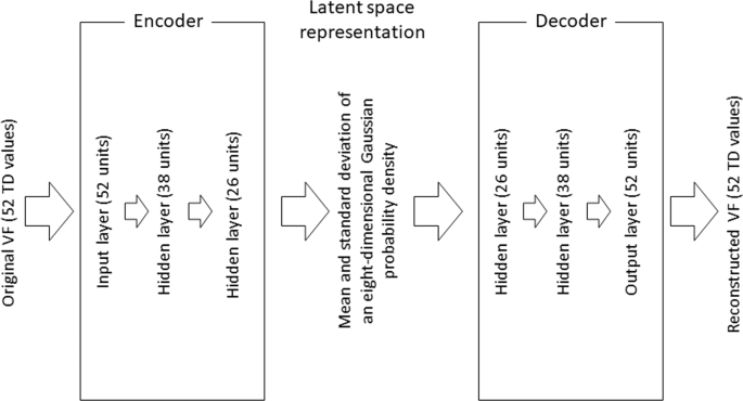
AUTOENCODER The structure of the VAE model is shown in Fig. 1. This was built using the training dataset. The encoder is a 1-layer neural network consisting of 52 units (for each of the 52

TD values). This encoder is connected to 2 hidden layers consisting of 38 and 26 units, and is then represented by the mean and standard deviation of an eight-dimensional Gaussian

probability density in the latent space. The decoder reconstructs the 52 TD (TDVAE) values through a further 2 hidden layers and 1 output layer, which represents the reconstructed VF. This

VAE model was optimized by maximizing the sum of the negative reconstruction loss, which is derived from the difference between the input VFs and reconstructed VFs and the Kullback–Leibler

divergence between the distributions. mTDVAE was calculated as the mean of 52 the TDVAE values. In the VAE calculation, TD values were scaled to between 0 and 1 (before encoder), and then

re-scaled back (after decoder) to the original values. STATISTICAL ANALYSIS ANALYSIS WITH TEST-RETEST DATASET ‘Test’ VFs in testing dataset 1 were reconstructed using the trained VAE. Then

the difference between mTD values in the first VF (the ‘test’ VF) and the VAE-reconstructed first VF (the ‘test’ VF) was calculated. In addition, the difference between mTD values in the

first VF (the ‘test’ VF) and in the second VF (the ‘retest’ VF) was calculated. The relationship between these two difference values was investigated. MTD TREND ANALYSIS Using testing

dataset 2, progression measured over all ten VFs (VF1–10) was regarded as a surrogate for true progression. The consistency of mTD trend analysis results was evaluated using the following

measures, following our previous reports23,24: * (1) Proportion of both progressing (PBP) was calculated as a surrogate measure for true-positive rate; i.e., where progression was

significant in VF1-10 and also in shorter VFs (from VF1-9 to VF1-3). * (2) Proportion of both not progressing (PBNP) was calculated as a surrogate measure for true negative rate; where

progression in the complete series of VFs (VF1-10) was deemed “not significant”, and progression also “not significant” in shorter subsets of VFs (from VF1-9 to VF1-5). * (3) Proportion of

inconsistent progression (PIP) was calculated as a surrogate measure for the false positive rate; classification based on the shorter series of VFs (from VF1-9 to VF1-5) was judged to be

“significant” but progression in the complete series of VFs (VF1-10) was “not significant.” Further, mTD trend analysis was carried out using mTD values from the 1st to the 3rd VFs (VF1-3)

of each patient, and the mTD values of the 10th VF test were predicted. The same procedure was carried out using the mTD values in longer series: VF1-4, VF1-5, VF1-6, VF1-7, VF1-8 and VF1-9,

and the mTD values of 10th VFs were predicted every time. In OLSLR, the regression line is decided so that the sum of squared residuals in the regression becomes minimum. In contrast, in a

weighted linear regression analysis, the regression line is decided so that the sum of squared weighted residuals becomes minimum. To investigate the usefulness of the VAE for mTD trend

analyses, the absolute difference between mTD and mTDVAE values were calculated for each VF in testing dataset 2 and a weighted mTD trend analysis (mTDVAE trend analysis) was performed using

the difference as a weight in the regression (calculated as 1/absolute difference between mTD and mTDVAE values). Then, similarly to the standard mTD trend analysis, PBP, PBNP, PIP values

and also prediction accuracy were calculated using the mTDVAE trend analysis and compared to those with the unweighted mTD trend analysis. BINOMIAL PLR The detailed calculation of the

binomial PLR method is described in our previous report23,24. As detailed in our previous reports23,24, the assumption in PLR is that VF damage progresses linearly over time, similarly to

the MD trend analysis27,28,29, where the null hypothesis was that the slope of VF progression was equal to 0. With this null hypothesis, slope p-values of coefficient from the linear

regression can vary between the values of 0 and 1, where the numbers of test points with a p-value less than an arbitrary value would follow the binomial distribution. When this null

hypothesis was rejected, a slope coefficient of zero is considered unlikely a result of random chance. In the current study, following our previous reports22,23,24, the significance of the

entire VF progression was assessed using the four cut-off p values of 0.025, 0.05, 0.075, and 0.1. To represent these four p-values, the median p value was used30,31. A VF sequence was

regarded as “significant” when the p-value calculated with the binomial PLR was <0.025; otherwise, it was “not significant.” Using this approach, PBP, PBNP, PIP, and the time to first

detect a significant progression were calculated, similarly to the MD trend analysis. Using the PBP, PBNP and PIP summary measurements, the accuracy of the weighted binomial PLR (binomial

PLRVAE) was compared where the weight values were calculated as (1/absolute difference between TD and TDVAE values). In addition, the number of VFs required to detect significant progression

for the first time was calculated for each method. The sensitivity of each method to detect progression was assessed using Kaplan-Meier survival analysis and compared using the logrank

test. RESULTS TESTING DATASET 1 (ANALYSIS WITH TEST-RETEST DATASET) Demographic summary data of testing dataset 1 is shown in Table 1. The mTD value in the second VF was significantly

related both with the mTD value in the first VF (R = 0.83, p < 0.001, linear model) and mTDVAE derived from the 1st VFs (R = 0.84, p < 0.001). There was a significant positive

relationship between the difference between mTD values in the first VF and the mTDVAE values derived from the first VF and the difference between mTD values in the first VF and mTD values in

the second VF (R = 0.76, p < 0.001, Fig. 2). A significant relationship was not observed for FL (p = 0.81), FP (p = 0.55) or FN (p = 0.53) in the first VF. TESTING DATASET 2 (MTD TREND

ANALYSIS) Demographic summary data of testing dataset 2 is shown in Table 2. Baseline mTD, follow-up period between VF1 and VF10, and mTD progression rate were − 6.9 ± 6.3 [Mean ± Standard

Deviation] dB, 5.4 ± 1.1 years, and − 0.26 ± 0.46 dB/year, respectively. There was a significant relationship between the mTD and mTDVAE (p < 0.001, linear mixed model where random

effects were subject and number of VF).The PBP values with the standard unweighted mTD trend analysis and the weighted mTDVAE trend analysis are presented in Fig. 3. PBP values were 0.33,

0.41, 0.55, 0.75, 0.78, 0.87, and 0.90 from VF1-3 to VF1-9 with the mTD trend analysis, respectively, whereas they were 0.41, 0.67, 0.68, 0.72, 0.75, 0.71, and 0.76, respectively, with the

mTDVAE trend analysis. There was no significant difference in the PBP values of the two methods (P = 0.14, paired Wilcoxon test). The PBNP values with the unweighted mTD trend analysis and

the weighted mTDVAE trend analysis, are presented in Fig. 4. These values were 0.77, 0.77, 0.79, 0.82, 0.83, 0.87, and 0.92 from VF1-3 to VF1-9 with the mTD trend analysis, respectively,

whereas they were 0.78, 0.79, 0.81, 0.84, 0.86, 0.88, and 0.92, respectively, with the mTDVAE trend analysis. There was a significant difference in the PBNP values of the two methods (P = 

0.016, paired Wilcoxon test). The PIP values with the unweighted mTD trend analysis and weighted mTDVAE trend analysis, are presented in Fig. 5. These values were 0.0096, 0.021, 0.028,

0.024, 0.026, 0.022, and 0.023 from VF1-3 to VF1-9 with the mTD trend analysis, respectively, whereas they were 0.016, 0.011, 0.024, 0.033, 0.038, 0.061, and 0.064, respectively, with mTDVAE

trend analysis. There was no significant difference in the PIP values of the two methods (P = 0.16, paired Wilcoxon test). Figure 6 shows the comparison of mean squared prediction errors

between the unweighted mTD trend analysis and the weighted mTDVAE trend analysis. The errors were 58.7, 22.7, 12.6, 6.8, 4.7, 3.4, and 2.3 from VF1-3 to VF1-9 with the unweighted mTD trend

analysis, respectively, whereas they were 53.0, 19.8, 11.0, 6.5, 4.6, 3.2, and 2.3, respectively, with the mTDVAE trend analysis. There was a significant difference in errors from the two

methods (P = 0.031, paired Wilcoxon test). BINOMIAL PLR Figures 7, 8, and 9 show the comparisons of PBP, PBNP, and PIP values between the unweighted binomial PLR and weighted binomial

PLRVAE. The PBP values with binomial PLR ranged from 0.07 with VF1-3 to 0.81 with VF1-9, whereas those with binomial PLRVAE were between 0.21 with VF1-3 and 0.81 with VF1-9. The PBNP values

with binomial PLR ranged from 0.89 with VF1-7 to 0.95 with VF1-3, whereas those with binomial PLRVAE were between 0.84 with VF1-3 and 0.92 with VF1-8 and VF1-9, respectively. The PIP values

with binomial PLR ranged from 0.088 with VF1-9 to 0.51 with VF1-3, whereas those with binomial PLRVAE were between 0.090 with VF1-9 and 0.44 with VF1-3, respectively. There was not a

significant difference in the values of PBNP and PIP (p = 0.078 and 0.078, paired Wilcoxon test), whereas the values of PBP with binomial PLRVAE were significantly higher than those with

binomial PLR (p = 0.016, paired Wilcoxon test). Kaplan-Meier survival analysis and the logrank test indicated that the binomial PLRVAE detected significantly more progressing eyes than the

binomial PLR, (P < 0.0001) (Fig. 10). The time to classification of progression with each method was: 6.8 ± 2.9 (mean ± SD) years with mTD trend analysis, 4.3 ± 1.6 years with binomial

PLRVAE, and 4.7 ± 1.5 years with binomial PLR. DISCUSSION In the current study, a VAE model was developed using 82,433 VFs from 16,836 eyes of 9,139 subjects. The usefulness of this method

to improve the reproducibility of mTD measurements, and accuracy of trend analyses was investigated. VF reproducibility, in the form of test-retest mTD, was better using the VAE-derived

measurement (mTDVAE). The accuracy of mTD trend analysis and binomial PLR was enhanced using the mTDVAE; further, the sensitivity of binomial PLR was improved using mTDVAE. VF data are

inherently associated with measurement noise. In the current study, it was suggested that it is beneficial to consider mTDVAE in addition to mTD itself to predict the mTD value in the retest

VF. In particular, when mTDVAE took a larger value than the value of mTD in the first VF, mTD in the second VF tended to be larger than that in the first VF (suggesting the measurement may

be under-estimated). Conversely when mTDVAE derived from the first VF took a smaller value than the value of mTD, mTD value in the second VF tended to be smaller than that in the first VF

(suggesting the measurement may be over-estimated). Visual field measurement noise has a considerable effect on the accuracy of trend analyses6. In the current study, the average mTD

progression rate was −0.26 ± 0.46 dB/year. From real world clinics, Heijl _et al_. reported a VF progression rate of −0.80 dB/year, in 583 patients with open angle glaucoma, where the

average baseline MD value was −10.0 dB (median)32. In 587 patients with glaucoma, De Moraes _et al_. reported a −0.45 dB/year VF progression rate when the baseline MD value was equal to −7.1

 dB (mean)33. As shown by the analysis of the test-retest data in the current study, mTDVAE was related to mTD in the second VF after an adjustment for mTD in the first VF. This implies that

the accuracy of mTD trend analyses may be improved by considering the difference between mTDVAE and mTD. Indeed, the current results suggested that applying a weighted linear regression

using these differences as weights yielded more accurate predictions compared to the unweighted approach (see Fig. 6). We previously reported that applying least absolute shrinkage and

selection operator (LASSO) in linear regression resulted in much more accurate prediction error than the conventional mTD trend analysis34. Similarly, we also reported that Variational

Bayesian Linear Regression, in which the mTD trend analysis was optimized by considering the temporal and spatial VF defect patterns, enabled more accurate predictions of VF progression

compared to the conventional mTD trend analysis35,36. The magnitude of increase in prediction accuracy with the mTDVAE trend analysis is smaller than that observed in these previously

reported models. However, accuracy may be further improved by combining the current approach with these other regression models. There have been previous studies which suggested the

usefulness of non-linear regression, instead of liner regression, in VF trend analysis17,37,38,39,40. However we previously investigated the usefulness of the application of such non-linear

regression approaches (exponential, quadratic, and logistic regressions, as well as robust regression models) in VF trend analysis41. The experiment setting was very similar to that in the

current study: future VF was predicted using prior (shorter) VF sequences. As a result, it was suggested no improvement of the prediction error was obtained by any method, compared to the

conventional ordinary least squares linear regression. In addition, there is another non-negligible drawback of the application of the non-linear regression model at the clinical settings;

significance of the obtained non-linear curve cannot be calculated. Thus, although it may be of interest to further investigating the usefulness of applying the current approach to such

non-linear regression models, the clinical usefulness would be limited. There was not a significant difference between PBP (Fig. 3) and PIP (Fig. 4) values for the standard mTD trend

analysis and the proposed mTDVAE trend analysis. This suggests that these methods have similar sensitivity and false positive rates when diagnosing progression. On the other hand, PBNP value

with the mTDVAE trend analysis, however, was significantly higher than that with the conventional mTD trend analysis (Fig. 5), suggesting the new approach has better specificity. We

previously reported that applying the binomial test to PLR resulted in improved PBP and PIP values compared to standard mTD trend analysis. We further investigated whether using a weighted

PLR (with weights equal to the differences between TD and TDVAE values at each test point) is beneficial in binomial PLR. Sensitivity (Fig. 7) and the false positive rate (Fig. 8) were not

significantly different between the two methods, however significantly higher PBNP values were obtained with binomial PLRVAE compared to binomial PLR (Fig. 9). Furthermore, the sensitivity

to detect progression was significantly better with binomial PLRVAE than with binomial PLR (Fig. 10). In the current study, there was not a significant positive relationship between the

difference between mTD and the mTDVAE values, and FL, FP and FN. FL, FP and FN are the indices currently used to assess the reliability of measured VF. More specifically, FL, FP, FN is

thought to indicates test reliability and vision fixation, “trigger-happy” patients, and inattention during an examination25,42,43,44,45,46. While some past studies have reported on the

usefulness of these indices47,48, more recent studies have suggested their limitations; for instance, FLs can also result from the mislocalization of the blind spot49 and fixational

instability can be found even in well trained observers43,50. A high FN rate is reported to be associated with the amount of field loss as well as threshold reproducibility4. The VF noise

estimated by the difference between mTD and the mTDVAE values cannot be explained by these VF reliability indices, but we speculate that this is because of these limitations of these

reliability measures. Another possible approach would be further investigating this issue using a microperimetry with retinal tracking, such as MP-3 (Nidel Co.Ltd., Aichi, Japan), because

more accurate assessment of VF can be conducted preventing the effect of eye movement (mis-location)51. One of the limitations of the current study is a lack of results from the HFA 10-2

test. Recent studies have revealed that it is recommended to measure the HFA 10-2 VF in addition to the HFA 24-252,53,54,55,56,57. In addition, damage to this area of the VF is more directly

associated with patients’ vision related to the quality of life58,59 A future study should be attempted shedding light on the usefulness of VAE in the HFA 10-2 test. In addition, various

spatial filter methods, such as60, have been reported which are other possible approach to reduce VF noise. It would be of interest to investigate the usefulness of them compared to VAE in a

future study. In addition, generative adversarial network (GAN)61 is further another possible deep learning approach to reduce noise in VF. In general, GAN generates images which look more

natural by human beings compared to VAE, however VF is not a material to be recognized the shape by human beings, so this merit may and may not be observed in VF. It would be of interest to

compare the usefulness of VAE and GAN in a future study. In conclusion, we developed a method to reconstruct the VF measurement using a deep learning method. The approach appears to be

useful to predict MD value in the retested VF and also to improve the reliability of MD trend analyses and also binomial PLR. REFERENCES * Quigley, H. A. & Broman, A. T. The number of

people with glaucoma worldwide in 2010 and 2020. _Br. J. Ophthalmol._ 90, 262–7 (2006). Article  CAS  PubMed  PubMed Central  Google Scholar  * Flammer, J., Drance, S. M., Fankhauser, F.

& Augustiny, L. Differential light threshold in automated static perimetry. Factors influencing short-term fluctuation. _Arch. Ophthalmol._ 102, 876–9 (1984). Article  CAS  PubMed 

Google Scholar  * Flammer, J., Drance, S. M. & Zulauf, M. Differential light threshold. Short- and long-term fluctuation in patients with glaucoma, normal controls, and patients with

suspected glaucoma. _Arch. Ophthalmol._ 102, 704–6 (1984). Article  CAS  PubMed  Google Scholar  * Bengtsson, B. & Heijl, A. False-negative responses in glaucoma perimetry: indicators of

patient performance or test reliability? _Invest. Ophthalmol. Vis. Sci._ 41, 2201–4 (2000). CAS  PubMed  Google Scholar  * Henson, D. B., Evans, J., Chauhan, B. C. & Lane, C. Influence

of fixation accuracy on threshold variability in patients with open angle glaucoma. _Invest. Ophthalmol. Vis. Sci._ 37, 444–50 (1996). CAS  PubMed  Google Scholar  * Jansonius, N. M. On the

accuracy of measuring rates of visual field change in glaucoma. _Br. J. Ophthalmol._ 94, 1404–5 (2010). Article  CAS  PubMed  Google Scholar  * Kingma DP, Welling M: Auto-Encoding

Variational Bayes. arXiv 2013, 1312. * Rezende, D. J., Mohamed, S. & Wierstra, D. Stochastic Backpropagation and Approximate Inference in Deep Generative Models. _arXiv_ 1401 (2014). *

Chen, S., Meng, Z. & Zhao, Q. Electrocardiogram Recognization Based on Variational AutoEncoder, Machine Learning and Biometrics. IntechOpen 2018, 7634. * Aggarwal, C .C. Neural Networks

and Deep Learning: A Textbook. Nerlin, Germany: Springer, 2018. * Asaoka, R. _et al_.: Improving structure-function relationship in glaucomatous visual fields by using a Deep Learning-based

noise reduction approach. Ophthalmology Glaucoma (In press. 2020). * Fitzke, F. W., Hitchings, R. A., Poinoosawmy, D., McNaught, A. I. & Crabb, D. P. Analysis of visual field progression

in glaucoma. _Br. J. Ophthalmol._ 80, 40–8 (1996). Article  CAS  PubMed  PubMed Central  Google Scholar  * Wild, J. M., Hussey, M. K., Flanagan, J. G. & Trope, G. E. Pointwise

topographical and longitudinal modeling of the visual field in glaucoma. _Invest. Ophthalmol. Vis. Sci._ 34, 1907–16 (1993). CAS  PubMed  Google Scholar  * Azarbod, P. _et al_. Validation of

point-wise exponential regression to measure the decay rates of glaucomatous visual fields. _Invest. Ophthalmol. Vis. Sci._ 53, 5403–9 (2012). Article  PubMed  Google Scholar  * Bryan, S.

R., Vermeer, K. A., Eilers, P. H., Lemij, H. G. & Lesaffre, E. M. Robust and censored modeling and prediction of progression in glaucomatous visual fields. _Invest. Ophthalmol. Vis.

Sci._ 54, 6694–700 (2013). Article  PubMed  Google Scholar  * O’Leary, N., Chauhan, B. C. & Artes, P. H. Visual field progression in glaucoma: estimating the overall significance of

deterioration with permutation analyses of pointwise linear regression (PoPLR). _Investig. Ophthalmol. Vis. Sci._ 53, 6776–84 (2012). Article  Google Scholar  * McNaught, A. I., Crabb, D.

P., Fitzke, F. W. & Hitchings, R. A. Modelling series of visual fields to detect progression in normal-tension glaucoma. _Graefes Arch. Clin. Exp. Ophthalmol._ 233, 750–5 (1995). Article

  CAS  PubMed  Google Scholar  * Viswanathan, A. C., Fitzke, F. W. & Hitchings, R. A. Early detection of visual field progression in glaucoma: a comparison of PROGRESSOR and STATPAC 2.

_Br. J. Ophthalmol._ 81, 1037–42 (1997). Article  CAS  PubMed  PubMed Central  Google Scholar  * Viswanathan, A. C. _et al_. Interobserver agreement on visual field progression in glaucoma:

a comparison of methods. _Br. J. Ophthalmol._ 87, 726–30 (2003). Article  CAS  PubMed  PubMed Central  Google Scholar  * Nouri-Mahdavi, K., Brigatti, L., Weitzman, M. & Caprioli, J.

Comparison of methods to detect visual field progression in glaucoma. _Ophthalmology_ 104, 1228–36 (1997). Article  CAS  PubMed  Google Scholar  * Yousefi, S. _et al_. Detection of

Longitudinal Visual Field Progression in Glaucoma Using Machine Learning. _Am. J. Ophthalmol._ 193, 71–9 (2018). Article  PubMed  Google Scholar  * Karakawa, A., Murata, H., Hirasawa, H.,

Mayama, C. & Asaoka, R. Detection of progression of glaucomatous visual field damage using the point-wise method with the binomial test. _PLoS One_ 8, e78630 (2013). Article  ADS  CAS 

PubMed  PubMed Central  Google Scholar  * Asano, S., Murata, H., Matsuura, M., Fujino, Y. & Asaoka, R. Early Detection of Glaucomatous Visual Field Progression Using Pointwise Linear

Regression With Binomial Test in the Central 10 Degrees. _Am. J. Ophthalmol._ 199, 140–9 (2019). Article  PubMed  Google Scholar  * Asano, S. _et al_. R A: Validating the Efficacy of the

Binomial Pointwise Linear Regression Method to detect Glaucoma Progression with Multi-central Database. _Br. J. Ophthalmol_. (In Press, 2020). * Anderson, D. R. & Patella, V. M.

_Automated Static Perimetry_. 2nd ed. St. Louis: Mosby, (1999). * Fujino, Y. _et al_. Japanese Archive of Multicentral Databases in Glaucoma Construction G: Evaluation of Glaucoma

Progression in Large-Scale Clinical Data: The Japanese Archive of Multicentral Databases in Glaucoma (JAMDIG). _Invest. Ophthalmol. Vis. Sci._ 57, 2012–20 (2016). Article  PubMed  Google

Scholar  * Crabb, D. P. & Garway-Heath, D. F. Intervals between visual field tests when monitoring the glaucomatous patient: wait-and-see approach. _Invest. Ophthalmol. Vis. Sci._ 53,

2770–6 (2012). Article  PubMed  Google Scholar  * McNaught, A. I., Crabb, D. P., Fitzke, F. W. & Hitchings, R. A. Visual field progression: comparison of Humphrey Statpac2 and pointwise

linear regression analysis. _Graefes Arch. Clin. Exp. Ophthalmol._ 234, 411–8 (1996). Article  CAS  PubMed  Google Scholar  * Russell, R. A., Crabb, D. P., Malik, R. & Garway-Heath, D.

F. The relationship between variability and sensitivity in large-scale longitudinal visual field data. _Invest. Ophthalmol. Vis. Sci._ 53, 5985–90 (2012). Article  PubMed  Google Scholar  *

van de Wiel, M. A., Berkhof, J. & van Wieringen, W. N. Testing the prediction error difference between 2 predictors. _Biostatistics_ 10, 550–60 (2009). Article  PubMed  Google Scholar  *

Fisher RA: Statistical methods for research workers. Breakthroughs in statistics: Springer, pp. 66–70 (1992). * Heijl, A., Buchholz, P., Norrgren, G. & Bengtsson, B. Rates of visual

field progression in clinical glaucoma care. _Acta Ophthalmol._ 91, 406–12. (2013). Article  PubMed  Google Scholar  * De Moraes, C. G. _et al_. Risk factors for visual field progression in

treated glaucoma. _Arch. Ophthalmol._ 129, 562–8 (2011). Article  PubMed  Google Scholar  * Fujino, Y., Murata, H., Mayama, C. & Asaoka, R. Applying “Lasso” Regression to Predict Future

Visual Field Progression in Glaucoma Patients. _Invest. Ophthalmol. Vis. Sci._ 56, 2334–9 (2015). Article  PubMed  Google Scholar  * Murata, H., Araie, M. & Asaoka, R. A new approach to

measure visual field progression in glaucoma patients using variational bayes linear regression. _Invest. Ophthalmol. Vis. Sci._ 55, 8386–92 (2014). Article  PubMed  Google Scholar  *

Murata, H. _et al_. Validating Variational Bayes Linear Regression Method With Multi-Central Datasets. _Invest. Ophthalmol. Vis. Sci._ 59, 1897–904 (2018). Article  PubMed  PubMed Central 

Google Scholar  * Pathak, M., Demirel, S. & Gardiner, S. K. Reducing Variability of Perimetric Global Indices from Eyes with Progressive Glaucoma by Censoring Unreliable Sensitivity

Data. _Transl. Vis. Sci. Technol._ 6, 11 (2017). Article  PubMed  PubMed Central  Google Scholar  * Nouri-Mahdavi, K., Hoffman, D., Gaasterland, D. & Caprioli, J. Prediction of visual

field progression in glaucoma. _Invest. Ophthalmol. Vis. Sci._ 45, 4346–51 (2004). Article  PubMed  Google Scholar  * Caprioli, J. _et al_. A method to measure and predict rates of regional

visual field decay in glaucoma. _Invest. Ophthalmol. Vis. Sci._ 52, 4765–73 (2011). Article  PubMed  Google Scholar  * Bengtsson, B., Patella, V. M. & Heijl, A. Prediction of

glaucomatous visual field loss by extrapolation of linear trends. _Arch. Ophthalmol._ 127, 1610–5 (2009). Article  PubMed  Google Scholar  * Humphrey Field Analyzer series 700 serveice guide

section 1, (1994). * Vingrys, A. J. & Demirel, S. The effect of fixational loss on perimetric thresholds and reliability. Perimetry Update 1992/93. Amsterdam: Kugler Publications

(1992). * Demirel, S. & Vingrys, A. J. Eye Movements During Perimetry and the Effect that Fixational Instability Has on Perimetric Outcomes. _J. Glaucoma_ 3, 28–35 (1994). Article  CAS 

PubMed  Google Scholar  * Newkirk, M. R., Gardiner, S. K., Demirel, S. & Johnson, C. A. Assessment of false positives with the Humphrey Field Analyzer II perimeter with the SITA

Algorithm. _Invest. Ophthalmol. Vis. Sci._ 47, 4632–7 (2006). Article  PubMed  Google Scholar  * Fankhauser, F., Spahr, J. & Bebie, H. Some aspects of the automation of perimetry.

_Survey Ophthalmol._ 22, 131–41. (1977). * Johnson, C. A., Sherman, K., Doyle, C. & Wall, M. A comparison of false-negative responses for full threshold and SITA standard perimetry in

glaucoma patients and normal observers. _J. Glaucoma_ 23, 288–92 (2014). Article  PubMed  Google Scholar  * McMillan, T. A., Stewart, W. C. & Hunt, H. H. Association of reliability with

reproducibility of the glaucomatous visual field. _Acta Ophthalmol._ 70, 665–70 (1992). Article  CAS  Google Scholar  * Katz, J. & Sommer, A. Screening for glaucomatous visual field

loss. _Eff. patient reliability. Ophthalmol._ 97, 1032–7 (1990). CAS  Google Scholar  * Sanabria, O., Feuer, W. J. & Anderson, D. R. Pseudo-loss of fixation in automated perimetry.

_Ophthalmology_ 98, 76–8 (1991). Article  CAS  PubMed  Google Scholar  * Demirel S, Vingrys AJ: Fixational instability during perimetry and the blindspot monitor. Amsterdam: Perimetry Update

1992/1993. Kugler Publications, (1992). * Matsuura, M. _et al_. Evaluating the Usefulness of MP-3 Microperimetry in Glaucoma Patients. _Am. J. Ophthalmol._ 187, 1–9 (2018). Article  PubMed

  Google Scholar  * De Moraes, C. G. _et al_. 24-2 Visual Fields Miss Central Defects Shown on 10-2 Tests in Glaucoma Suspects, Ocular Hypertensives, and Early Glaucoma. _Ophthalmology_ 124,

1449–56 (2017). Article  PubMed  Google Scholar  * Grillo, L. M. _et al_. The 24-2 Visual Field Test Misses Central Macular Damage Confirmed by the 10-2 Visual Field Test and Optical

Coherence Tomography. _Transl. Vis. Sci. Technol._ 5, 15 (2016). Article  PubMed  PubMed Central  Google Scholar  * Park, H. Y., Hwang, B. E., Shin, H. Y. & Park, C. K. Clinical Clues to

Predict the Presence of Parafoveal Scotoma on Humphrey 10-2 Visual Field Using a Humphrey 24-2 Visual Field. _Am. J. Ophthalmol._ 161, 150–9 (2016). Article  PubMed  Google Scholar  *

Hangai, M., Ikeda, H. O., Akagi, T. & Yoshimura, N. Paracentral scotoma in glaucoma detected by 10-2 but not by 24-2 perimetry. _Jpn. J. Ophthalmol._ 58, 188–96 (2014). Article  PubMed 

Google Scholar  * Traynis, I. _et al_. Prevalence and nature of early glaucomatous defects in the central 10 degrees of the visual field. _JAMA Ophthalmol._ 132, 291–7 (2014). Article 

PubMed  PubMed Central  Google Scholar  * Park, S. C. _et al_. Parafoveal scotoma progression in glaucoma: humphrey 10-2 versus 24-2 visual field analysis. _Ophthalmology_ 120, 1546–50

(2013). Article  PubMed  Google Scholar  * Murata, H. _et al_. Identifying areas of the visual field important for quality of life in patients with glaucoma. _PLoS One_ 8, e58695 (2013).

Article  ADS  CAS  PubMed  PubMed Central  Google Scholar  * Sumi, I., Shirato, S., Matsumoto, S. & Araie, M. The relationship between visual disability and visual field in patients with

glaucoma. _Ophthalmology_ 110, 332–9 (2003). Article  PubMed  Google Scholar  * Strouthidis, N. G. _et al_. Structure and function in glaucoma: The relationship between a functional visual

field map and an anatomic retinal map. _Investig. Ophthalmol. Vis. Sci._ 47, 5356–62 (2006). Article  Google Scholar  * Goodfellow I, _et al_.: Generative adversarialnets. Advances in neural

information processing systems 2014:2672-80. Download references ACKNOWLEDGEMENTS Supported in part by Grants 25861618 (HM) and 19H01114 and 18KK0253 and 26462679 (RA) from the Ministry of

Education, Culture, Sports, Science and Technology of Japan, and grants from Suzuken Memorial Foundation and Mitsui Life Social Welfare Foundation. AUTHOR INFORMATION AUTHORS AND

AFFILIATIONS * Department of Ophthalmology, Graduate School of Medicine and Faculty of Medicine, The University of Tokyo, Tokyo, 113-8655, Japan Ryo Asaoka, Hiroshi Murata, Shotaro Asano, 

Masato Matsuura & Yuri Fujino * Seirei Hamamatsu General Hospital, Shizuoka, 432-8558, Japan Ryo Asaoka * Seirei Christpther University, Shizuoka, 433-8558, Japan Ryo Asaoka * Department

of Ophthalmology, Graduate School of Medical Sciences, Kitasato University, Kanagawa, 252-0374, Japan Masato Matsuura, Yuri Fujino & Nobuyuki Shoji * Department of Ophthalmology, Osaka

University Graduate School of Medicine, Osaka, 565-0871, Japan Atsuya Miki * Department of Ophthalmology, Shimane University Faculty of Medicine, Shimane, 693-8501, Japan Masaki Tanito *

Division of Ophthalmology, Matsue Red Cross Hospital, Shimane, Japan Masaki Tanito * Department of Ophthalmology, Ehime University Graduate School of Medicine, Ehime, 791-0295, Japan Shiro

Mizoue * Department of Ophthalmology, Kyoto Prefectural University of Medicine, Kyoto, 602-8566, Japan Kazuhiko Mori * Department of Ophthalmology, Yamaguchi University Graduate School of

Medicine, Yamaguchi, 755-0046, Japan Katsuyoshi Suzuki * Department of Ophthalmology, Kagoshima University Graduate School of Medical and Dental Sciences, Kagoshima, 890-0075, Japan Takehiro

Yamashita * Department of Ophthalmology, University of Yamanashi Faculty of Medicine, Yamanashi, 409-3898, Japan Kenji Kashiwagi Authors * Ryo Asaoka View author publications You can also

search for this author inPubMed Google Scholar * Hiroshi Murata View author publications You can also search for this author inPubMed Google Scholar * Shotaro Asano View author publications

You can also search for this author inPubMed Google Scholar * Masato Matsuura View author publications You can also search for this author inPubMed Google Scholar * Yuri Fujino View author

publications You can also search for this author inPubMed Google Scholar * Atsuya Miki View author publications You can also search for this author inPubMed Google Scholar * Masaki Tanito

View author publications You can also search for this author inPubMed Google Scholar * Shiro Mizoue View author publications You can also search for this author inPubMed Google Scholar *

Kazuhiko Mori View author publications You can also search for this author inPubMed Google Scholar * Katsuyoshi Suzuki View author publications You can also search for this author inPubMed 

Google Scholar * Takehiro Yamashita View author publications You can also search for this author inPubMed Google Scholar * Kenji Kashiwagi View author publications You can also search for

this author inPubMed Google Scholar * Nobuyuki Shoji View author publications You can also search for this author inPubMed Google Scholar CONTRIBUTIONS Conceived and designed the

experiments: Y.F., H.M., R.A. Performed the experiments: R.A., S.A., Analyzed the data: R.A., S.A. Contributed reagents/materials/analysis tools: M.M., Y.F., H.M., A.M., M.T., S.M., K.M.,

K.S., T.Y., K.K., N.S., Wrote the paper: Y.F., R.A., R.A., H.M., S.A., M.M., Y.F., A.M., M.T., S.M., K.M., K.S., T.Y., K.K. and N.S. reviewed the manuscript. CORRESPONDING AUTHOR

Correspondence to Ryo Asaoka. ETHICS DECLARATIONS COMPETING INTERESTS The authors declare no competing interests. ADDITIONAL INFORMATION PUBLISHER’S NOTE Springer Nature remains neutral with

regard to jurisdictional claims in published maps and institutional affiliations. RIGHTS AND PERMISSIONS OPEN ACCESS This article is licensed under a Creative Commons Attribution 4.0

International License, which permits use, sharing, adaptation, distribution and reproduction in any medium or format, as long as you give appropriate credit to the original author(s) and the

source, provide a link to the Creative Commons license, and indicate if changes were made. The images or other third party material in this article are included in the article’s Creative

Commons license, unless indicated otherwise in a credit line to the material. If material is not included in the article’s Creative Commons license and your intended use is not permitted by

statutory regulation or exceeds the permitted use, you will need to obtain permission directly from the copyright holder. To view a copy of this license, visit

http://creativecommons.org/licenses/by/4.0/. Reprints and permissions ABOUT THIS ARTICLE CITE THIS ARTICLE Asaoka, R., Murata, H., Asano, S. _et al._ The usefulness of the Deep Learning

method of variational autoencoder to reduce measurement noise in glaucomatous visual fields. _Sci Rep_ 10, 7893 (2020). https://doi.org/10.1038/s41598-020-64869-6 Download citation *

Received: 18 September 2019 * Accepted: 08 February 2020 * Published: 12 May 2020 * DOI: https://doi.org/10.1038/s41598-020-64869-6 SHARE THIS ARTICLE Anyone you share the following link

with will be able to read this content: Get shareable link Sorry, a shareable link is not currently available for this article. Copy to clipboard Provided by the Springer Nature SharedIt

content-sharing initiative