News Reader.info

ABSTRACT The exchange of trace gases between the atmosphere and the ocean plays a key role in the Earth’s climate. Fluxes at the air-sea interface are affected mainly by wind blowing over

the ocean and seawater temperature and salinity changes. This study aimed to quantify the use of CO\(_{2}\) partial pressure (pCO\(_{2}\)) measurements at different depths (1, 5, and 10 m)

in ocean surface layers to determine CO\(_{2}\) fluxes (FCO\(_{2}\)) and to investigate the impacts of wind-sheltered and wind-exposed regions on the carbon budget. Vertical profiles of

temperature, salinity, and pCO\(_{2}\) were considered during a daily cycle. pCO\(_{2}\) profiles exhibited relatively high values during sunny hours, associated with relatively high sea

temperatures. However, the largest FCO\(_{2}\) corresponded with higher wind speeds. Estimated fluxes between measurements at 1 and 10 m depths decreased by 71% in the sheltered region and

44% in the exposed region. According to the SOCAT dataset, at a depth of 5 m, the Atlantic basin emits approximately 0.29 Tg month\(^{-1}\) of CO\(_{2}\) to the atmosphere; nevertheless, our

estimates suggest that FCO\(_{2}\) at the surface is 12.02 Tg month\(^{-1}\), which is 97.6% greater than that at 5 m depth. Therefore, future studies should consider sampling depth to

adequately estimate the FCO\(_{2}\). SIMILAR CONTENT BEING VIEWED BY OTHERS ENHANCED OCEAN CO2 UPTAKE DUE TO NEAR-SURFACE TEMPERATURE GRADIENTS Article Open access 25 October 2024 SURFACE

WATER CO2 VARIABILITY IN THE GULF OF MEXICO (1996–2017) Article Open access 23 July 2020 NATURAL VARIABILITY IN AIR–SEA GAS TRANSFER EFFICIENCY OF CO2 Article Open access 30 June 2021

INTRODUCTION Earth’s oceans are important carbon sinks, removing an estimated 25%1,2,3 to 30%4 of the total CO\(_{2}\) emissions from the atmosphere. Gas exchange across the air-sea

interface is driven mainly by wind blowing over the sea surface5 and changes in seawater temperature and salinity. The latter changes influence the solubility of dissolved gases and thus the

amount available for air–sea exchange6. Understanding the associated processes is essential for quantifying air-sea CO\(_{2}\) fluxes (FCO\(_{2}\)), their variability, and their response to

different forcing mechanisms. Some studies have estimated air-sea FCO\(_{2}\) using in-situ measurements at depths ranging from 1 to 5 m7,8,9 and from 5 to 7 m10,11,12 and below 7 m13;

these are all considered surface measurements. Coastal regions and continental/island shelves play important roles in the global carbon cycle. Compared with the global average, carbon

fixation ratios are greater in these regions9,14,15 due to several factors such as large temperature changes, biological activity, mixing, strong tidal forces, and freshwater inputs

(e.g.,13,16,17). These factors lead to greater spatial and seasonal variations in surface water pCO\(_{2}\) in coastal waters than in open ocean waters. Some authors have estimated

FCO\(_{2}\) for Atlantic coastal regions; however, the global carbon budget has not fully considered coastal waters due to the reduced number of local and regional studies18,19. Warm oceanic

wakes are regional phenomena characterized by relatively warm surface waters. This occurs due to the interaction between incoming winds and high mountainous islands, resulting in weaker

winds and a clearing of clouds on the leeward side. This leads to intense solar radiation reaching the sea surface, forming a warm oceanic wake. This phenomenon is detectable from space on

Madeira Island (northeastern Atlantic Ocean) and can extend 100 km offshore during summer. In this wind-sheltered region, the sea surface temperature can be 4 \(^{\circ }\)C higher than that

of the surrounding oceanic waters (e.g.,20). The waters are strongly stratified concerning temperature; the gradient is greater in the first 20 m, creating a daily thermocline21.

Conversely, the open ocean shows enhanced vertical mixing and greater mixed-layer depth, especially on the island’s southwestern coast22 (the exposed region considered in this study). The

complexity of the processes influencing air-sea exchange and seasonal and spatial variability is among the greatest obstacles to obtaining real values of FCO\(_{2}\). In this regard, our

study highlights the implications of using partial pressure of CO\(_{2}\) (pCO\(_{2}\)) measurements at different depths in the first layers of the ocean to estimate FCO\(_{2}\). In

addition, the impact of regional phenomena on the carbon budget is also investigated. To attain our goal, in-situ measurements at different surface depths (1 m, 5 m, and 10 m) were used to

analyse the difference in carbon fluxes between a wind-sheltered region and an exposed region. Following the introduction, the paper is organized as follows: “Results” presents the results,

including observations. “Discussion” discusses and summarizes the main findings. “Methods” describes the datasets and methods. RESULTS Considering that FCO\(_{2}\) varies seasonally and

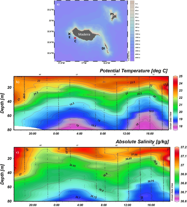
spatially with the water characteristics and wind, this section focuses on the vertical structure of temperature and salinity measured in the wind-sheltered region (Fig. 1); atmospheric and

water pCO\(_{2}\) and normalized pCO\(_{2}\) (NpCO\(_{2}\)) (Fig. 2); and wind speed (in the lower atmosphere) and calculated FCO\(_{2}\) (Fig. 3) in the wind-sheltered and exposed regions.

In general, the water column in the wind-sheltered region was stratified, with temperatures being higher at the surface and decreasing with depth (Fig. 1b). The values ranged between 24 and

24.5 \(^{\circ }\)C at the surface and between 18 and 19 \(^{\circ }\)C at a depth of 80 m. The impact of solar radiation is noticeable at the first 10 m, with variations occurring only

during sunny hours (23 to 24.5 \(^{\circ }\)C). A distinct influence is perceptible at depths between 10 and 40 m, adding a cycle oscillation at the isotherms in the water column. This

oscillation could be related to the tidal cycle. During flood tide (HT, Fig. 1b), the isotherms stretched to greater depths and became more visible during the late afternoon with

temperatures of approximately 23.5\(^{\circ }\)C at a depth of 40 m. During ebb tide (LT), colder waters rise to shallow depths (20 m depth). Below 40 m, the isotherms seem to respond only

to the cycle oscillation. The salinity (Fig. 1c) had a similar pattern of variation with temperature throughout the water column. Therefore, salinity gradients were observed instead of a

homogeneous layer in the first 10 m. Additionally, a low-salinity water mass at the surface during the flood tide, contrasted with the higher salinity during the ebb tide. In the

wind-sheltered region, the atmospheric pCO\(_{2}\) presented daily variations of less than 2 \(\upmu\)atm (Fig. 2a–c). The values varied by 1.6 \(\upmu\)atm during sunny hours (between  

403.7 \(\upmu\)atm at 1700 UTC and  405.3 \(\upmu\)atm at 1120 UTC, the minimum and maximum, respectively, over three days; Fig. 2a–c). Between day and night (Fig. 2a), the values decreased

during the night (404.8 \(\upmu\)atm at 2336 UTC to 404.5 \(\upmu\)atm at 0555 UTC), increased after sunrise (404.8 \(\upmu\)atm at 0720 UTC to 405.3 \(\upmu\)atm at 1120 UTC) and decreased

again after the peak heat hour (1300 UTC). The water pCO\(_{2}\) varied with sunny hours; in particular, higher values occurred during the day (0800 UTC and 1700 UTC; Fig. 2e), when higher

temperatures were recorded (Fig. 1a). This variation is visible at all depths and on all three days (Fig. 2e–g), with less amplitude at a depth of 10 m (blue line in Fig. 2). The water

pCO\(_{2}\) values ranged from approximately 406 to 465 \(\upmu\)atm at 1 m, from 407 to 460 \(\upmu\)atm at 5 m and from 396 to 430 \(\upmu\)atm at 10 m (at 0800 UTC and 1700 UTC,

respectively). The discrepancy in the depths from 1 to 5 m is lower (approximately 5 \(\upmu\)atm; 1%) than that from 5 to 10 m (approximately 20 \(\upmu\)atm; 4%). In the exposed region

(Fig. 2h), this discrepancy is identical among the three depths, at 2.29% and 1.97% for the 1 to 5 m and 5 to 10 m depths, respectively. After normalizing the water pCO\(_{2}\) to a constant

temperature of 24 \(^{\circ }\)C (Fig. 2i–l) to account for the contribution of physical and biological processes to the observed variability, the activity of NpCO\(_{2}\) throughout the

day was maintained, but in general, the values increased at depths of 5 and 10 m. This occurred in both regions, i.e., the sheltered and exposed regions. At 5 m depth (red line), the

NpCO\(_{2}\) values were equal to or even greater than those at 1 m depth (black line) on all three days. The values at 10 m depth (blue line) also changed and were more elevated; moreover,

on August 16th, the NpCO\(_{2}\) values at 10 m were similar to those at 1 m depth. The discrepancy among the three depths decreased in both regions, with less variation in the NpCO\(_{2}\)

values in the exposed region. The calculated fluxes (Fig. 3) were greater in the exposed region (maximum of 1.46 mmol m\(^{-2}\) day\(^{-1}\); Fig. 3h) than in the sheltered region (maximum

of 0.69 mmol m\(^{-2}\) day\(^{-1}\); Fig. 3e–g), at all depths. In general, in the sheltered region, the FCO\(_{2}\) behaviour was consistent with that of pCO\(_{2}\); i.e., higher values

of pCO\(_{2}\) indicate greater fluxes (Fig. 3f,g). However, on August 16th (Fig. 3e), FCO\(_{2}\) showed significant variations related to wind variability (Fig. 3a–d). Positive peaks in

FCO\(_{2}\) occurred in response to wind speed intensification (e.g., 0.1 mmol m\(^{-2}\) day\(^{-1}\) at 1.7 ms\(^{-1}\) at 0000 UTC; 0.39 mmol m\(^{-2}\) day\(^{-1}\) at 3.4 ms\(^{-1}\) at

0400 UTC). In contrast, when the wind speed decreased, the FCO\(_{2}\) also decreased (e.g., 0.03 mmol m\(^{-2}\) day\(^{-1}\) at 0.9 ms\(^{-1}\) at 0130 UTC; 0.11 mmol m\(^{-2}\)

day\(^{-1}\) at 2.1 ms\(^{-1}\) at 0600 UTC). These peaks occurred with lower pCO\(_{2}\) during the nighttime at depths of 1 and 5 m. After sunrise (0900 UTC), another FCO\(_{2}\) peak was

observed (0.42 mmol m\(^{-2}\) day\(^{-1}\)) with a higher wind speed (3.7 ms\(^{-1}\)) and an increase in pCO\(_{2}\) (423 \(\upmu\)atm; Fig. 2a). At the 10 m depth the FCO\(_{2}\) was

close to zero, except during the morning (0725–1130 UTC), when it increased, followed by a decrease in pCO\(_{2}\). This is the only time that the ocean behaved as a sink for atmospheric

CO\(_{2}\). Comparison of the FCO\(_{2}\) (calculated with pCO\(_2\) measurements) in both regions at the same time revealed that the values decreased by approximately 12% in the sheltered

region (0.26–0.23 mmol m\(^{-2}\) day\(^{-1}\)) and 6% in the exposed region (1.46 to 1.38 mmol m\(^{-2}\) day\(^{-1}\)), at depths from 1 to 5 m. However, considering the higher peaks of

FCO\(_{2}\) in the sheltered region (0.39 to 0.28 mmol m\(^{-2}\) day\(^{-1}\)), the decrease could reach 28% at depths between 1 and 5 m and 99% between 1 and 10 m. In the exposed region at

10 m, the decrease reached 44% compared with that at 1 m depth. DISCUSSION A precise assessment of spatial and seasonal variability8 and a greater characterization of coastal regions14 are

fundamental for improving our knowledge of the impacts of oceanographic and meteorological processes on the carbon cycle. To date, most scientific studies have focused on using shipboard

CO\(_{2}\) measurements to calculate air-sea fluxes (i.e., FCO\(_{2}\)) directly11,12,13,23, extrapolating the values in time and space8, or even using parameterizations based on surface

water properties10. Although the data contain original CO\(_{2}\) surface water measurements, such measurements are usually made several meters below the surface, which can be a source of

potential error in FCO\(_{2}\) calculations6,24. This potential error arises from the assumption of vertical homogeneity within the mixed layer25. Therefore, if vertical concentration

gradients exist in the mixed layer, as is the case in the wind-sheltered region with stratified temperature and salinity layers (Fig. 1a,b), then underway seawater is not representative of

the surface boundary layer, which could create a global sampling bias26. Despite pronounced seasonal variations17, the North Atlantic has been recognized as one of the largest ocean sinks of

CO\(_{2}\), especially at subtropical latitudes (e.g.,8,27,28,29)23, studied the seasonal variability in CO\(_{2}\) in the Northeast Atlantic Ocean between the northwestern African coast

and the open-ocean waters of the North Atlantic subtropical gyre. The results showed that during 2019, the region behaved as an annual CO\(_{2}\) sink of -2.65 ± 0.44 Tg CO\(_{2}\)

year\(^{-1}\). However, during the warm months, this entire region acted as a CO\(_{2}\) source23,30,31. In our study, which was performed in summer, the sheltered and exposed regions acted

predominantly as a source of CO\(_{2}\), in agreement with the literature. The higher values of pCO\(_{2}\) during sunny hours (in the wind-sheltered region, Fig. 2a–c) are consistent with

the highest sea surface temperature (Fig. 1a) and vice versa. This result aligns with the study by26, which investigated the influence of solar heat-trapping and near-surface warming on

CO\(_{2}\) gas exchange. The study noted that the existence of a warm oceanic surface layer creates a net asymmetry in CO\(_{2}\) transfer between the ocean and atmosphere. The warming and

cooling cycle of the upper ocean leads to a decrease in CO\(_{2}\) invasion and an increase in CO\(_{2}\) evasion, impacting the net daily exchange of CO\(_{2}\), which is consistent with

our findings (in the wind-sheltered region; Figs. 1 and  2). Similarly32, reported that in subtropical waters, CO\(_{2}\) transfer conditions were governed primarily by temperature.

According to our results, after normalizing the pCO\(_{2}\) to a constant temperature of 24 \(^{\circ }\)C an increase in the values was observed (Fig. 2e–h) principally in the deepest

layers. This should be ascribed to vertical mixing processes driven by tidal effects, bringing up the coldest and remineralized deeper waters, as happens on the salinity of the deepest

layers (Fig. 1b). On the other hand, at night, the pCO\(_{2}\) concentrations decreased, and concurrently with higher wind speeds, the FCO\(_{2}\) increased (see 0400 UTC; Fig. 3a),

indicating that CO\(_{2}\) was transferred to the atmosphere. Reference33 affirms that higher winds to a static \(\triangle pCO_{2}\) (without thermodynamic forces) can act synergistically

on the trend in FCO\(_{2}\). Although not investigated in this work, thermal and haline skin effects affect the FCO\(_{2}\) calculation. These effects should be considered in more complete

future research. Despite being only a few millimeters thick at the sea surface and generally weaker than the thermal effects6, the thermal skin effect increases oceanic global uptake25.

Additionally, according to6, the salty skin effect accounts for approximately one-sixth of the thermal effect. Nevertheless, it is also important to note the difference in FCO\(_{2}\)

between the study regions. Although both acted as sources, FCO\(_{2}\) varied from 1.46 mmol \(m^{-2}d^{-1}\) in the exposed region to 0.26 mmol \(m^{-2}d^{-1}\) in the sheltered region,

corresponding to 82% of the difference at the same time. Some global ocean-atmosphere FCO\(_{2}\) studies have excluded coastal regions8,10,11. Recently, the Integrated Ocean Carbon Research

report34 affirmed that coastal and marginal seas remain understudied. Laruelle et al.18 reported that CO\(_{2}\) fluxes could become 40% more intense in ice-free surface regions than in

exposed regions. In14, it was determined that the inclusion of coastal zones increased the estimated global ocean CO\(_{2}\) sinks by 57% at high latitudes and by 15% at mid-latitudes, while

CO\(_{2}\) emissions from the ocean to the atmosphere increased by 13% in tropical and subtropical regions. Our results showed the underestimated impact of using pCO\(_{2}\) measurements at

different ocean depths on FCO\(_{2}\) estimation at the local scale. However, what impact could such underestimation have on the Atlantic Ocean basin? In this sense, the FCO\(_{2}\) was

calculated for the Atlantic North Basin using the underestimation values obtained in this study at the exposed region (2.29% and 1.97% for the 1 m and 10 m depths, respectively). Figure 4

shows the sea surface temperature (Fig. 4a) and the wind speed (Fig. 4b) in the Atlantic North Basin. According to this figure, the temperature of the sea surface (Fig. 4a) increased from

the north (\(\sim\) 12 \(^{\circ }\)C; mid-latitudes) to the south (\(\sim\) 27 \(^{\circ }\)C; tropics). On the African coast and surrounding the archipelagos of Madeira and the Canary

Islands, the values were lower (between 20 and 24 \(^{\circ }\)C) than those at the same latitude (27 \(^{\circ }\)C; e.g., 32\(^{\circ }\) N). The wind speed (Fig. 4b), on the other hand,

had greater values (11 ms\(^{-1}\)) close to these regions. In turn, the weakest winds (until 2 ms\(^{-1}\) ) can be observed in the northeast, close to the Azores and south of the Cape

Verde archipelagos. The FCO\(_{2}\) estimates at depths of 1, 5, and 10 m are shown in Fig. 5a–c, respectively. Throughout August, at the mid-latitudes, the ocean acted as a CO\(_{2}\) sink

(blue in Fig. 5), while in the tropics, the ocean acted as a source (red in Fig. 5) of CO\(_{2}\). The fluxes were almost zero in the subtropics; despite the higher temperatures reported in

this region (in the range of 24–26 \(^{\circ }\)C), the winds were weaker. Here, the African coast and surrounding archipelagos of Madeira and the Canary Islands were exceptions; the

orographic winds exhibited greater values, between \(\sim\) 9 and 11 ms\(^{-1}\), and although the sea surface temperatures ranged from 22 to 24 \(^{\circ }\)C, the FCO\(_{2}\) displayed

higher values for the Atlantic basin. The lowest sea surface temperature, between 15 and 17 \(^{\circ }\)C, and the stronger winds (\(\sim\) 9 ms\(^{-1}\)) in the northwestern part of the

mid-latitudes created an intense CO\(_{2}\) sink region in the ocean. Considering the depths of the measurements, the FCO\(_{2}\) values changed significantly between the surface and depths

of 5 and 10 m. Although the pattern persisted, the values decreased substantially from the surface to a depth of 10 m. In the latter scenario, some regions of the tropical ocean transitioned

from source to sink. According to the SOCAT dataset, at a depth of 5 m, the Atlantic basin emits approximately 0.29 Tg month\(^{-1}\) of CO\(_{2}\) to the atmosphere. The estimated

FCO\(_{2}\) (with pCO\(_2\) measurements) at 1 m depth, 12.02 Tg month\(^{-1}\), is 97.6% greater than that estimated at 5 m depth, despite the minor difference (2.29%) in pCO\(_2\), which

was found in our study at the same depths. Observation of the FCO\(_{2}\) estimated with the pCO\(_2\) at 10 m revealed that this behaviour reversed, and the FCO\(_{2}\) in the Atlantic

Basin decreased to 9.85 Tg month\(^{-1}\). FCO\(_{2}\) values change significantly with the depths of in-situ measurements, indicating the significance of proper measurement acquisition.

More studies should be performed to confirm the trends in different regions, and modelling studies should consider this important variability in flux calculations. Future studies should also

continue to evaluate differences in pCO\(_2\) at different depths. METHODS Identifying and quantifying near-surface gradients in trace gas concentrations is challenging. Several instruments

were used to capture the response of the ocean’s surface layer to atmospheric forcing. Data acquisition was performed during a summer campaign in 2021 (16–23 August) onboard a vessel of

opportunity. On August 16 (24 h), 20 (12 h) and 23 (12 h), oceanographic and meteorological data were collected every 2 h at station C (Fig. 1); at station E, data were collected on August

23. In the ocean, temperature and salinity were measured, while air temperature and wind speed were measured in the lower atmosphere. pCO\(_{2}\) was recorded in the ocean and

lower-atmosphere. In the ocean, data were acquired using a conductivity, temperature, and depth profiler (pumped CTD, SeaBird-19). The CTD was measured at 4 Hz, and a total of 13 vertical

profiles were obtained. The acquisition was carried out using Seaterm software, and the processing included a set of SBE Data Processing routines (Sea-Bird Electronics), as detailed in21.

Furthermore, the partial pressure of CO\(_{2}\) gas dissolved in water was measured with a pCO\(_{2}\) sensor (submersible sensor, Pro Oceanus) using infrared detection at a sample rate of 1

second and a resolution of 0.01 ppm. For a consistent concentration, the sensor was preequilibrated under seawater conditions for a 30-min period. To achieve equilibrium between the

pCO\(_{2}\) membrane and the seawater at depth, the sensor was lowered at a rate of 3 m/min. The data were classified into three depths using the mean: 0–1 m, 5–6 m, and 10–11 m. The

standard deviation was calculated. pCO\(_{2}\) was also measured in the lower atmosphere by pumping air instead of seawater. An SBE-37 sensor, used to record temperature, salinity, and

pressure, was combined with the pCO\(_{2}\) sensor, and samples were processed at a sampling rate of 1 second. Air-sea fluxes of carbon dioxide are commonly determined by first measuring

partial pressure gradients between the ocean surface and lower atmosphere and then multiplying them by a parameter called the gas transfer velocity. The CO\(_{2}\) fluxes were determined

using Eq. (1): $$\begin{aligned} FCO_{2} = 0.24 S k \triangle pCO_{2} \end{aligned}$$ (1) where 0.24 is a conversion factor to express data in mmol m\(^{-2}\) day\(^{-1}\); S is the

solubility of CO\(_{2}\) in seawater; and \(\bigtriangleup pCO_{2}\) is the difference between the seawater and low atmosphere (pCO\(_{2,sw}\) - pCO\(_{2,atm}\)). Positive fluxes indicate

that the ocean acts as a source of CO\(_{2}\) to the atmosphere, while negative fluxes indicate that the ocean acts as an atmospheric CO\(_{2}\) sink. The gas transfer velocity is usually

parameterized as a function of the wind speed. Wind does not directly control gas transfer; more precisely, gas transfer is governed by complex boundary layer processes. However, most of

these boundary layer processes are strongly influenced by wind, and on a global scale, wind can be used as the sole environmental forcing. The parameterization of35 was used in this study,

with k (cm h\(^{-1}\)) being the gas transfer rate expressed in Eq. (2): $$\begin{aligned} k = 0.251 <U^2> \left( \frac{Sc}{660} \right) ^{-0.5} \end{aligned}$$ (2) where U is the wind

speed (ms\(^-1\)) and Sc is the Schmidt number (kinematic viscosity of seawater) divided by the gas diffusion coefficient. This parameterization contributes to the uncertainty of the flux.

The relationship between wind speed and gas exchange was studied by35, and the uncertainty reached 20% for a basin-scale application. Woolf et al.36 also analysed this uncertainty using

calculations referenced to 2010 and concluded that a realistic estimate is approximately 9%. Woolf et al.36 also referred to temperature gradients as a source of uncertainty. To remove the

thermal effect on daily variation, pCO\(_{2}\) was normalized to a constant temperature of 24 \(^{\circ }\)C using a mean coefficient of 0.0423 \(^{\circ }\)C\(^{-1}\), determined

experimentally by32 (and confirmed by37) for a North Atlantic surface water sample and using Eq. 3: $$\begin{aligned} NpCO_{2} = (pCO_{2})_{obs} \times exp[ 0.0423 (24-T_{obs})]

\end{aligned}$$ (3) In the atmosphere, vertical profiles were determined via atmospheric radiosondes (DFM-09, GRAW Radiosondes). The atmospheric radiosondes measured profiles of air

temperature (accuracy < 0.2 \(^{\circ }\)C), air pressure (accuracy < 0.3 hPa), wind speed (accuracy < 0.2 ms\(^-1\)) and wind direction. All the sensors were calibrated. The

FCO\(_{2}\) was estimated for the North Atlantic Basin using sea surface pCO\(_{2}\) from the Surface Ocean CO2 Atlas (SOCAT v202238), global ocean monthly temperature and salinity (in-situ

measurements39), global ocean monthly mean sea surface wind from Copernicus (scatterometer data and model40) and global hourly surface pressure data (reanalysis41). The details of the data

processing are presented below. The SOCAT pCO\(_{2}\) measurements span 1963 through 2021. These types of measurements are often collected from the underway seawater intake of research

vessels for a depth range of 2–7 m (our study treats this range of depths as 5 m). To adjust the pCO\(_{2}\) values for 2021, an increment of 1.7 \(\upmu\)atm/year was computed using the

monthly mean carbon dioxide data from the Mauna Loa Observatory, Hawaii (https://gml.noaa.gov/ccgg/trends/data.html). Using the actualized pCO\(_{2}\) values, a linear interpolation was

carried out throughout the entire North Atlantic Ocean using the SST grid, which has a spatial resolution of 0.5\(^{\circ }\). Afterwards, the underestimation values obtained in this study

(2.29% and 1.97% for 1 m and 10 m depths, respectively) were assumed to be valid for the North Atlantic and applied to the interpolated pCO\(_{2}\) values, considering only August. Finally,

the FCO\(_{2}\) was calculated using Eq. (1) and the wind product. DATA AVAILIBILITY The datasets used and/or analysed during the current study are available from the corresponding author

upon reasonable request. REFERENCES * Le Quéré, C. _et al._ Global Carbon Budget 2018. _Earth Syst. Sci. Data_ 10, 2141–2194. https://doi.org/10.5194/essd-10-2141-2018 (2018). Article  ADS 

Google Scholar  * Friedlingstein, P. _et al._ Global Carbon Budget 2019. _Earth Syst. Sci. Data_ 11, 1783–1838. https://doi.org/10.5194/essd-11-1783-2019 (2019). Article  ADS  Google Scholar

  * Fay, A. R. _et al._ SeaFlux: harmonization of air-sea CO2 fluxes from surface pCO2 data products using a standardized approach. _Earth Syst. Sci. Data_ 13, 4693–4710.

https://doi.org/10.5194/essd-13-4693-2021 (2021). Article  ADS  Google Scholar  * Gruber, N. _et al._ The oceanic sink for anthropogenic CO 2 from 1994 to 2007. _Science_ 363, 1193–1199.

https://doi.org/10.1126/science.aau5153 (2019). Article  ADS  PubMed  CAS  Google Scholar  * Le Quéré, C. _et al._ Global Carbon Budget 2016. _Earth Syst. Sci. Data_ 8, 605–649.

https://doi.org/10.5194/essd-8-605-2016 (2016). Article  ADS  Google Scholar  * Woolf, D. K., Land, P. E., Shutler, J. D., Goddijn-Murphy, L. M. & Donlon, C. J. On the calculation of

air-sea fluxes of CO 2 in the presence of temperature and salinity gradients. _J. Geophys. Res. Oceans_ 121, 1229–1248. https://doi.org/10.1002/2015JC011427 (2016). Article  ADS  CAS  Google

Scholar  * Bakker, D. C. E., Etcheto, J., Boutin, J. & Merlivat, L. Variability of surface water f CO 2 during seasonal upwelling in the equatorial Atlantic Ocean as observed by a

drifting buoy. _J. Geophys. Res. Oceans_ 106, 9241–9253. https://doi.org/10.1029/1999JC000275 (2001). Article  ADS  CAS  Google Scholar  * Takahashi, T. _et al._ Climatological mean and

decadal change in surface ocean pCO2, and net sea-air CO2 flux over the global oceans. _Deep Sea Res. Part II_ 56, 554–577. https://doi.org/10.1016/j.dsr2.2008.12.009 (2009). Article  ADS 

CAS  Google Scholar  * Shadwick, E. _et al._ Seasonal variability of dissolved inorganic carbon and surface water pCO2 in the Scotian Shelf region of the Northwestern Atlantic. _Mar. Chem._

124, 23–37. https://doi.org/10.1016/j.marchem.2010.11.004 (2011). Article  CAS  Google Scholar  * Telszewski, M. _et al._ Estimating the monthly pCO2 distribution in the North Atlantic using

a self-organizing neural network. _Biogeosciences_ 6, 1405–1421. https://doi.org/10.5194/bg-6-1405-2009 (2009). Article  ADS  CAS  Google Scholar  * Watson, A. J. _et al._ Revised estimates

of ocean-atmosphere CO2 flux are consistent with ocean carbon inventory. _Nat. Commun._ 11, 4422. https://doi.org/10.1038/s41467-020-18203-3 (2020). Article  ADS  PubMed  PubMed Central 

CAS  Google Scholar  * Macovei, V. A., Callies, U., Calil, P. H. R. & Voynova, Y. G. Mesoscale Advective and Biological Processes Alter Carbon Uptake Capacity in a Shelf Sea. _Front.

Mar. Sci._ 9. https://doi.org/10.3389/fmars.2022.827075 (2022). * Curbelo-Hernández, D., González-Dávila, M. & Santana-Casiano, J. M. The carbonate system and air-sea CO2 fluxes in

coastal and open-ocean waters of the Macaronesia. _Front. Mar. Sci._ 10. https://doi.org/10.3389/fmars.2023.1094250 (2023). * Borges, A. V., Delille, B. & Frankignoulle, M. Budgeting

sinks and sources of CO 2 in the coastal ocean: Diversity of ecosystems counts. _Geophys. Res. Lett._ 32. https://doi.org/10.1029/2005GL023053 (2005). * Cai, W.-J., Dai, M. & Wang, Y.

Air-sea exchange of carbon dioxide in ocean margins: A province-based synthesis. _Geophys. Res. Lett._ 33, L12603. https://doi.org/10.1029/2006GL026219 (2006). Article  ADS  CAS  Google

Scholar  * Simpson, J. H. & Sharples, J. _Introduction to the Physical and Biological Oceanography of Shelf Seas_ (Cambridge University Press, 2012). * Laruelle, G. G. _et al._ Global

high-resolution monthly pCO2 climatology for the coastal ocean derived from neural network interpolation. _Biogeosciences_ 14, 4545–4561. https://doi.org/10.5194/bg-14-4545-2017 (2017).

Article  ADS  CAS  Google Scholar  * Laruelle, G. G., Lauerwald, R., Pfeil, B. & Regnier, P. Regionalized global budget of the CO 2 exchange at the air-water interface in continental

shelf seas. _Global Biogeochem. Cycles_ 28, 1199–1214. https://doi.org/10.1002/2014GB004832 (2014). Article  ADS  CAS  Google Scholar  * Landschützer, P., Laruelle, G. G., Roobaert, A. &

Regnier, P. A uniform pCO2 climatology combining open and coastal oceans. _Earth Syst. Sci. Data_ 12, 2537–2553. https://doi.org/10.5194/essd-12-2537-2020 (2020). Article  ADS  Google

Scholar  * Caldeira, R., Groom, S., Miller, P., Pilgrim, D. & Nezlin, N. Sea-surface signatures of the island mass effect phenomena around Madeira Island. _Northeast Atlantic. Remote

Sens. Environ._ 80, 336–360. https://doi.org/10.1016/S0034-4257(01)00316-9 (2002). Article  ADS  Google Scholar  * Azevedo, C. C., Camargo, C. M. L., Alves, J. & Caldeira, R. M. A.

Convection and Heat Transfer in Island (Warm) Wakes. _J. Phys. Oceanogr._ 51, 1187–1203. https://doi.org/10.1175/JPO-D-20-0103.1 (2021). Article  ADS  Google Scholar  * Alves, J. M.,

Caldeira, R. M. & Miranda, P. M. Dynamics and oceanic response of the Madeira tip-jets. _Q. J. R. Meteorol. Soc._ 146, 3048–3063. https://doi.org/10.1002/qj.3825 (2020). Article  ADS 

Google Scholar  * Curbelo-Hernández, D., González-Dávila, M., González, A., González-Santana, D. & Santana-Casiano, J. CO2 fluxes in the Northeast Atlantic Ocean based on measurements

from a surface ocean observation platform. _Sci. Total Environ._ 775, 145804. https://doi.org/10.1016/j.scitotenv.2021.145804 (2021). Article  PubMed  CAS  Google Scholar  * Rödenbeck, C.

_et al._ Global surface-ocean pCO2 and sea-air CO2 flux variability from an observation-driven ocean mixed-layer. _Ocean Sci._ 9, 193–216. https://doi.org/10.5194/os-9-193-2013 (2013).

Article  ADS  CAS  Google Scholar  * Robertson, J. E. & Watson, A. J. Thermal skin effect of the surface ocean and its implications for CO2 uptake. _Nature_ 358, 738–740.

https://doi.org/10.1038/358738a0 (1992). Article  ADS  CAS  Google Scholar  * McNeil, Craig L. & Merliva, L. The warm oceanic surface layer: Implications for CO2 fluxes and surface gas

measurements. _Geophys. Res. Lett._ 23, 3575–3578 (1996). * Sabine, C. L. _et al._ The Oceanic Sink for Anthropogenic CO 2. _Science_ 305, 367–371. https://doi.org/10.1126/science.1097403

(2004). Article  ADS  PubMed  CAS  Google Scholar  * Landschützer, P., Gruber, N., Bakker, D. C. E. & Schuster, U. Recent variability of the global ocean carbon sink. _Global Biogeochem.

Cycles_ 28, 927–949. https://doi.org/10.1002/2014GB004853 (2014). Article  ADS  CAS  Google Scholar  * Leseurre, C. _et al._ Ocean carbonate system variability in the North Atlantic

Subpolar surface water (1993-2017). _Biogeosciences_ 17, 2553–2577. https://doi.org/10.5194/bg-17-2553-2020 (2020). Article  ADS  CAS  Google Scholar  * Santana-Casiano, J. M.,

González-Dávila, M., Laglera Baquer, L. M. & Rodríguez Somoza, M. J. Carbon dioxide system in the Canary region during October 1995. _Sci. Mari._ 65, 41–50.

https://doi.org/10.3989/scimar.2001.65s141 (2001). * González-Dávila, M., Santana-Casiano, J. M., Rueda, M.-J., Llinás, O. & González-Dávila, E.-F. Seasonal and interannual variability

of sea-surface carbon dioxide species at the European Station for Time Series in the Ocean at the Canary Islands (ESTOC) between 1996 and 2000. _Global Biogeochem. Cycles_ 17.

https://doi.org/10.1029/2002GB001993 (2003). * Takahashi, T., Olafsson, J., Goddard, J. G., Chipman, D. W. & Sutherland, S. C. Seasonal variation of CO 2 and nutrients in the

high-latitude surface oceans: A comparative study. _Global Biogeochem. Cycles_ 7, 843–878. https://doi.org/10.1029/93GB02263 (1993). Article  ADS  CAS  Google Scholar  * Wanninkhof, R. _et

al._ Global ocean carbon uptake: magnitude, variability and trends. _Biogeosciences_ 10, 1983–2000. https://doi.org/10.5194/bg-10-1983-2013 (2013). Article  ADS  CAS  Google Scholar  *

Aricò, S. _et al._ Integrated Ocean Carbon Research: A Summary of Ocean Carbon Research, and Vision of Coordinated Ocean Carbon Research and Observations for the Next Decade. Tech. Rep.

https://doi.org/10.25607/h0gj-pq41(2021). * Wanninkhof, R. Relationship between wind speed and gas exchange over the ocean revisited. _Limnol. Oceanogr. Methods_ 12, 351–362.

https://doi.org/10.4319/lom.2014.12.351 (2014). Article  Google Scholar  * Woolf, D. K. _et al._ Key Uncertainties in the Recent Air-Sea Flux of CO2. _Global Biogeochem. Cycles_ 33,

1548–1563. https://doi.org/10.1029/2018GB006041 (2019). Article  ADS  CAS  Google Scholar  * Wanninkhof, R., Pierrot, D., Sullivan, K., Mears, P. & Barbero, L. Comparison of discrete and

underway CO2 measurements: Inferences on the temperature dependence of the fugacity of CO2 in seawater. _Mar. Chem._ 247, 104178. https://doi.org/10.1016/j.marchem.2022.104178 (2022).

Article  CAS  Google Scholar  * Bakker, D. C. E., Alin, S. R., Becker, M., Bittig, H. C., Castaño-Primo, R., Feely, R. A., Gkritzalis, T., Kadono, K., Kozyr, A., Lauvset, S.K., Metzl, N.,

Munro, D. R., Nakaoka, S. N., & Yukihiro, O’B D. Surface Ocean CO2 Atlas Database Version 2022 (SOCATv2022), https://doi.org/10.25921/1h9f-nb73 (2022). * Szekely, T., Gourrion, J.,

Pouliquen, S. & Reverdin, G. The CORA 52 dataset for global in situ temperature and salinity measurements: data description and validation. _Ocean Sci._ 15, 1601–1614.

https://doi.org/10.5194/os-15-1601-2019 (2019). Article  ADS  Google Scholar  * Polverari, F. _et al._ On High and Extreme Wind Calibration Using ASCAT. _IEEE Trans. Geosci. Remote Sens._

60, 1–10. https://doi.org/10.1109/TGRS.2021.3079898 (2022). Article  Google Scholar  * Hersbach, H., Bell, B., Berrisford, P., Biavati, G., Horányi, A., Muñoz Sabater, J., Nicolas, J.,

Peubey, C., Radu, R., Rozum, I., Schepers, D., Simmons, A., Soci, C., & Dee, D. Thépaut, J.-N. ERA5 hourly data on single levels from 1940 to present.

https://doi.org/10.24381/cds.adbb2d47 (2023). Download references ACKNOWLEDGEMENTS The authors would like to acknowledge the oceanographic group of the Oceanic Observatory of Madeira for

their participation in constructive discussions on the research subject. The Surface Ocean CO2 Atlas (SOCAT) is an international effort, endorsed by the International Ocean Carbon

Coordination Project (IOCCP), the Surface Ocean Lower Atmosphere Study (SOLAS) and the Integrated Marine Biosphere Research (IMBeR) program, to deliver a uniformly quality-controlled surface

ocean CO2 database. We thank the many researchers and funding agencies responsible for collecting data and quality control and their contributions to SOCAT. This work was financially

supported by the Oceanic Observatory of Madeira Project (M1420-01-0145- FEDER-000001-Observatório Oceânico da Madeira-OOM). Author C. C. Azevedo is currently funded by FCT

(SFRH/BD/147425/2019). AUTHOR INFORMATION AUTHORS AND AFFILIATIONS * Dom Luiz Institute, Faculty of Sciences, University of Lisbon, Lisbon, Portugal Cátia C. Azevedo & Rui M. A. Caldeira

* Oceanic Observatory of Madeira, ARDITI, Funchal, Portugal Cátia C. Azevedo & Rui M. A. Caldeira * Instituto de Oceanografía y Cambio Global, IOCAG, Universidad de Las Palmas de Gran

Canaria, 35017, Las Palmas de Gran Canaria, Spain Melchor González-Dávila, J. Magdalena Santana-Casiano & David González-Santana Authors * Cátia C. Azevedo View author publications You

can also search for this author inPubMed Google Scholar * Melchor González-Dávila View author publications You can also search for this author inPubMed Google Scholar * J. Magdalena

Santana-Casiano View author publications You can also search for this author inPubMed Google Scholar * David González-Santana View author publications You can also search for this author

inPubMed Google Scholar * Rui M. A. Caldeira View author publications You can also search for this author inPubMed Google Scholar CONTRIBUTIONS Data acquisition: C.C.A., M.G., J.M.S.,

R.M.A.C. Data analysis: C.C.A., M.G., J.M.S., D.G. Conceptualization, funding acquisition, and supervision: R.M.A.C., M.G. All authors reviewed the manuscript. CORRESPONDING AUTHOR

Correspondence to Cátia C. Azevedo. ETHICS DECLARATIONS COMPETING INTERESTS The authors declare no competing interests. ADDITIONAL INFORMATION PUBLISHER'S NOTE Springer Nature remains

neutral with regard to jurisdictional claims in published maps and institutional affiliations. RIGHTS AND PERMISSIONS OPEN ACCESS This article is licensed under a Creative Commons

Attribution 4.0 International License, which permits use, sharing, adaptation, distribution and reproduction in any medium or format, as long as you give appropriate credit to the original

author(s) and the source, provide a link to the Creative Commons licence, and indicate if changes were made. The images or other third party material in this article are included in the

article's Creative Commons licence, unless indicated otherwise in a credit line to the material. If material is not included in the article's Creative Commons licence and your

intended use is not permitted by statutory regulation or exceeds the permitted use, you will need to obtain permission directly from the copyright holder. To view a copy of this licence,

visit http://creativecommons.org/licenses/by/4.0/. Reprints and permissions ABOUT THIS ARTICLE CITE THIS ARTICLE Azevedo, C.C., González-Dávila, M., Santana-Casiano, J.M. _et al._ Impact of

sampling depth on CO\(_{2}\) flux estimates. _Sci Rep_ 14, 18476 (2024). https://doi.org/10.1038/s41598-024-69177-x Download citation * Received: 21 May 2024 * Accepted: 01 August 2024 *

Published: 09 August 2024 * DOI: https://doi.org/10.1038/s41598-024-69177-x SHARE THIS ARTICLE Anyone you share the following link with will be able to read this content: Get shareable link

Sorry, a shareable link is not currently available for this article. Copy to clipboard Provided by the Springer Nature SharedIt content-sharing initiative